Theory for Crystal Layer Raman

The Crystal Raman calculation models Raman scattering from a crystal slab or a multilayer stack. It combines the Raman tensors and phonon frequencies from a lattice-dynamical calculation with the optical electric fields calculated by the transfer matrix or scattering matrix methods described in Theory for Single Crystal Infrared Optics.

The method is intended for non-resonant Raman scattering from homogeneous Raman-active layers. The incident laser field and the reciprocal scattered field may be modified by refraction, reflection, absorption and interference within the stack. These effects are included by evaluating the electric fields throughout each Raman-active layer and integrating the Raman source over the layer thickness.

Geometry

The crystal layer uses the same laboratory frame as the single-crystal infrared calculation. The layer surface lies in the \(XY\) plane and the surface normal is the laboratory \(Z\) direction. The incident radiation lies in the \(XZ\) plane; p-polarised light is polarised in this plane and s-polarised light is polarised along \(Y\).

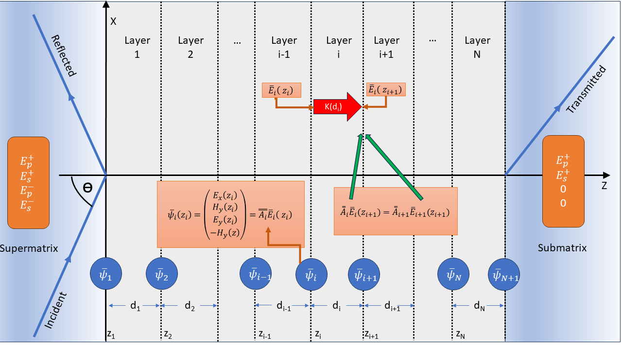
Fig. 55 Raman scattering from a multilayer system.

The laser is incident with angle \(\theta_L\). The detector may be on the superstrate side for backscattering or on the substrate side for forward scattering. The detected scattered radiation has frequency

(88)\[\nu_S = \nu_L - \nu_m\]

for Stokes scattering from mode \(m\). Here and in the numerical spectrum, \(\nu\) denotes wavenumber in cm⁻¹.

The signed collection angle specifies the outgoing ray’s x component. Automatic collection (Collection angle = -1 in saved GUI scripts) selects retro-backscattering on the superstrate side: \(\theta_{out}=-\theta_L\). On the substrate side it selects \(\theta_{out}=\theta_L\). An explicit positive angle equal to the incident angle selects specular backscattering. The reciprocal field is launched at \(-\theta_{out}\). At normal incidence these choices coincide; at oblique incidence they can produce different peak heights even with unchanged phonon frequencies.

The reciprocal-angle repair changes old oblique automatic-backscatter results. For example, the CASTEP ZnO 45° scenario’s dominant line retains its frequency but has about one third of its previous height. Explicit +45° collection recovers the former specular geometry; this is a geometry choice, not an intensity rescaling.

Layer Raman Amplitude

At a point \(z_s\) inside a Raman-active layer the scattering amplitude of mode \(m\) is

(89)\[A_m(z_s) \propto \mathbf{E}_S(z_s,\nu_S)^T \tensorbf{R}^{(m)}_{lab} \mathbf{E}_L(z_s,\nu_L)\]

where \(\mathbf{E}_L\) is the local electric field produced by the incident laser, \(\mathbf{E}_S\) is the reciprocal field associated with the detected scattered channel, and \(\tensorbf{R}^{(m)}_{lab}\) is the Raman tensor rotated into the laboratory frame. The transpose on \(\mathbf{E}_S\) is not a Hermitian conjugate; this is the usual reciprocity overlap used for Raman scattering from layered optical systems.

For a homogeneous layer \(\ell\), the layer amplitude is obtained by integrating through the layer thickness,

(90)\[A_{\ell m} = \int_{z_\ell}^{z_{\ell+1}} \mathbf{E}_S(z,\nu_S)^T \tensorbf{R}^{(m)}_{\ell,lab} \mathbf{E}_L(z,\nu_L)\,dz\]

PDielec evaluates this integral numerically using Gauss-Legendre quadrature points inside each Raman-active layer.

Optical Fields

The fields \(\mathbf{E}_L\) and \(\mathbf{E}_S\) are calculated from the same transfer matrix or scattering matrix machinery used for single-crystal infrared spectra. At optical laser frequencies the phonon contribution to the permittivity is not included; the high-frequency optical permittivity of each material is used for propagation through the stack.

The incident field \(\mathbf{E}_L(z,\nu_L)\) is calculated in the original multilayer system at the laser frequency. The scattered field is calculated at the shifted frequency \(\nu_S\). For backscattering the reciprocal field is launched from the superstrate side. For forward scattering it is launched from the substrate side, which is implemented by using the reversed stack and mapping each integration point to the corresponding position in that reversed system. With \(P=\operatorname{diag}(1,1,-1)\), the reversed stack uses \(P\varepsilon P\) in coordinates \((x,y,L-z)\); electric vectors are mapped back by \(P\) before contraction with the laboratory Raman tensor. Layer reversal alone is insufficient for anisotropic materials.

With the script option Approximate ES=True, the reciprocal detector field is instead evaluated once at the laser frequency and reused for all modes. The resolved collection geometry is retained. The incident field is reused only when the optical system and signed angle match those of the detector field. The default is False, which uses each mode’s Stokes frequency.

The detected channel can be p-polarised, s-polarised, or unpolarised. In the unpolarised case the p- and s-detected intensities are summed incoherently.

Raman Tensor Orientation

Reader tensors use \(R_\epsilon=\sqrt{V_{cell}}\partial\varepsilon_\infty/\partial Q_m\), with volume in \(\text{Å}^3\) and \(Q_m\) in Å times the square root of amu. They already contain the cell-volume normalization and enter RamanLayer directly. Raw Gaussian susceptibility derivatives require \(\partial\varepsilon=4\pi\partial\chi\); SI dimensionless susceptibility instead obeys \(\partial\varepsilon=\partial\chi_{SI}\).

The Raman tensor from the quantum mechanical calculation is defined in the crystal coordinate frame. If \(\tensorbf{G}\) maps vectors from the crystal frame to the laboratory frame,

(91)\[\mathbf{v}_{lab} = \tensorbf{G}\mathbf{v}_{crystal}\]

then the laboratory Raman tensor is

(92)\[\tensorbf{R}^{(m)}_{lab} = \tensorbf{G}\tensorbf{R}^{(m)}_{crystal}\tensorbf{G}^{T}\]

The rotation includes the surface orientation, specified by the layer Miller indices, and the azimuthal rotation about the laboratory \(Z\) axis. This allows the Raman intensity to be calculated as a function of azimuthal angle.

Combining Layers and Modes

For one mode, the layer amplitudes may be combined coherently or incoherently. Coherent combination sums amplitudes before squaring,

(93)\[I_m \propto \left|\sum_\ell A_{\ell m}\right|^2\]

whereas incoherent combination sums the layer intensities,

(94)\[I_m \propto \sum_\ell \left|A_{\ell m}\right|^2\]

This layer summation option is distinct from the Coherent or Incoherent choice in the layer table. The layer-table option controls optical propagation through that layer: whether the transfer/scattering matrix calculation retains phase interference from internal reflections, averages over phase, or treats a thick layer approximately. It therefore changes the optical fields \(\mathbf{E}_L\) and \(\mathbf{E}_S\) used in the Raman overlap.

The Layer combination option controls only how Raman amplitudes from different Raman-active layers are combined after those optical fields have been calculated. Use Incoherent intensities when separate active layers should contribute independent intensities, and use Coherent amplitudes only when Raman emission from those layers is expected to retain a fixed phase relationship and interfere.

The Depth coherence option is a third, more local coherence choice. It controls how Raman sources are combined through the thickness of each individual Raman-active layer. Coherent amplitude integrates the complex source amplitude before squaring. This is a raw constant-profile overlap: it supplies neither an explicit spatial phonon phase nor collective-state normalization. Interpreting it as one physical final state needs those additional specifications; small film thickness alone does not establish them:

(95)\[I_{\ell m} \propto \left| \int_{\ell} \mathbf{E}_S(z,\nu_S)^T \tensorbf{R}^{(m)}_{\ell,lab} \mathbf{E}_L(z,\nu_L)\,dz \right|^2 .\]

Incoherent intensity integrates the local intensity:

(96)\[I_{\ell m} \propto \int_{\ell} \left| \mathbf{E}_S(z,\nu_S)^T \tensorbf{R}^{(m)}_{\ell,lab} \mathbf{E}_L(z,\nu_L) \right|^2\,dz ,\]

which can describe spatially local source correlations. It also follows from a complete orthonormal spatial-state sum when the optical/tensor coupling and spectral weights are common to the included states; it does not require that each state itself be spatially localized. Film thickness alone does not determine phonon coherence. When Incoherent intensity is selected, PDielec also forces separate Raman-active layers to be combined as incoherent intensities, because there is then no well-defined layer amplitude to add coherently.

The mode intensity is then multiplied by the Stokes radiation and thermal factor,

(97)\[(\nu_L-\nu_m)^4\frac{n(\nu_m)+1}{\nu_m}\]

where \(n(\nu_m)\) is the Bose-Einstein occupation factor. The final spectrum is formed by applying Lorentzian broadening to each active mode,

(98)\[I(\Delta\nu) = \sum_m I_m \frac{\sigma_m}{(\Delta\nu-\nu_m)^2+\sigma_m^2}\]

where \(\sigma_m\) is the Lorentzian half-width at half maximum in cm⁻¹. This implemented line shape has integral \(\pi\) over the full wavenumber axis. Thus \(I_m\) is a line coefficient and its full integrated area is \(\pi I_m\), not \(I_m\). A unit-area Lorentzian requires division by \(\pi\). A spectral density on a different axis also needs the appropriate Jacobian; relabelling the frequency axis alone does not convert its units.

Crystal and powder calculations use the same scattered-frequency fourth-power weight. It is applied once per final phonon state, using its corrected frequency, including modal-pair, worker and contribution outputs. Raw optical amplitudes remain unweighted. This changes both the overall scale and relative line heights from the reduced crystal intensities produced before the September 2026 repair. Absolute experimental collection and cross-section constants are still omitted.

Only finite frequencies satisfying \(0<\nu_m<\nu_L\) and the acoustic cutoff contribute, independently of the scattered-field approximation. Negative frequencies remain available in phonon diagnostics as evidence of instability. Complex mechanical Raman tensors retain their phase through NAC mixing and EO addition; the EO susceptibility model remains the static electronic response.

Layer Phonon Frequencies

The NAC eigensolver uses Hartree atomic units: volume in Bohr cubed, masses in electron masses and Born charges in elementary-charge units. Its electrostatic prefactor is \(4\pi/V\). With SI charges and masses, the corresponding prefactor is \(1/(\epsilon_0 V)\) instead. Atomic-unit eigenvalues are converted to cm⁻¹ by dividing their signed square roots by Constants.wavenumber, the numerical factor \(100h c_{SI}/E_h\). An SI eigenvalue requires division by \(2\pi100c_{SI}\). These two conventions must not be mixed.

The optical field calculation and the active-layer vibrational calculation are separate parts of the model. The transfer or scattering matrix calculation determines the laser field and the reciprocal scattered field at optical frequencies. It does not, by itself, change the phonon frequencies. Any shift of an infrared-active Raman mode away from the bulk transverse-optic value must therefore be included in the phonon dynamical matrix used for the Raman-active layer.

For each Raman-active layer PDielec starts from the transverse-optic dynamical matrix, the mass-weighted Born charge tensor and the Raman tensor of the layer material. The phonon-induced polarisation is written as

(99)\[\mathbf{P}_{ph} = \frac{1}{V}\tensorbf{Z}^{mw}\mathbf{x}\]

where \(\mathbf{x}\) is the mass-weighted normal-coordinate displacement vector and \(V\) is the unit-cell volume used for the Born charges. A macroscopic electrostatic field generated by this polarisation gives an additional restoring-force term,

(100)\[\tensorbf{D}^{eff} = \tensorbf{D}^{TO} + \frac{1}{\epsilon_0 V} \left(\tensorbf{Z}^{mw}\right)^T \tensorbf{S}_{ph} \tensorbf{Z}^{mw}\]

where \(\tensorbf{S}_{ph}\) is the phonon-field screening tensor. Different choices of \(\tensorbf{S}_{ph}\) define the phonon-frequency model for the active layer. After the correction has been applied, \(\tensorbf{D}^{eff}\) is diagonalised and the resulting frequencies and eigenvectors are used to form the Raman spectrum. The Raman tensors are transformed consistently with the corrected eigenvectors when mode mixing is introduced by the macroscopic field correction.

PDielec provides four levels of treatment for the active-layer phonon frequencies. These levels should be regarded as separate approximations for the phonon problem, not as alternatives for solving the optical propagation problem.

TO — bulk TO frequencies (GUI label: TO)

No macroscopic phonon-field correction is applied:

(101)\[\tensorbf{S}_{ph}=\tensorbf{0}, \qquad \tensorbf{D}^{eff}=\tensorbf{D}^{TO}\]

This is appropriate for modes that are not infrared active, for calculations where the long-range electric field is deliberately neglected, or as a reference calculation. It is also the most direct comparison with a conventional Placzek Raman calculation using the bulk transverse-optic phonon frequencies.

Snell’s law — travelling-wave NAC correction (GUI label: Snell’s law or Snell’s law (EO))

The phonon is assigned the momentum carried by the Raman process. In the laboratory frame,

(102)\[\mathbf{q}_{ph}=\mathbf{k}_{L}-\mathbf{k}_{S}\]

where \(\mathbf{k}_{L}\) is the optical wave vector of the laser field in the active layer and \(\mathbf{k}_{S}\) is the wave vector of the emitted Stokes photon in the same layer. The direction \(\hat{\mathbf{q}}_{ph}=\mathbf{q}_{ph}/|\mathbf{q}_{ph}|\) is used in the usual non-analytic correction. After rotating the layer background permittivity into the laboratory frame, the screening tensor is

(103)\[\tensorbf{S}^{NAC}_{ph} = \frac{\hat{\mathbf{q}}_{ph}\hat{\mathbf{q}}_{ph}^{T}} {\hat{\mathbf{q}}_{ph}^{T} \tensorbs{\varepsilon}^{b}_{i,lab} \hat{\mathbf{q}}_{ph}}\]

The implemented geometry estimate uses \(n=\sqrt{\max(\operatorname{Tr}(\varepsilon_\infty)/3,1)}\) and \(\sin\theta_{int}=\sin\theta_{ext}/n\), assuming an air launch medium. It subtracts unit optical directions, omitting the finite Stokes/laser magnitude ratio. It supplies one direction for the layer’s NAC calculation, while the Raman overlap retains the full optical fields. This approximation can return the TO fallback for collinear forward collection; that fallback is not evidence that the physical finite-shift momentum vanishes.

Dominant mode — dominant Berreman eigenmode (GUI label: Dominant mode or Dominant mode (EO))

Instead of the macroscopic Snell’s-law estimate, the phonon wavevector direction is taken from the actual Berreman eigenvalue of the dominant forward-propagating optical mode in the active layer. The generalised transfer matrix (GTM) system is solved at the laser frequency \(\nu_L\) to obtain the four Berreman \(k_z\) eigenvalues of the layer; the transmitted-p eigenvalue is used for p-polarised incidence and the transmitted-s eigenvalue for s-polarised incidence. A second GTM solve at the collection geometry, also at the laser frequency, gives an approximate outgoing \(k_z\). The phonon momentum transfer in the reduced wavevector \((\zeta, 0, q_z)\) space is then

(104)\[\begin{split}\mathbf{q}_{ph} \propto \begin{pmatrix}\zeta_L - \zeta_S \\ 0 \\ q_{z,L} - q_{z,S}\end{pmatrix} \quad\text{(backscattering: } \zeta_L-\zeta_S,\; q_{z,L}+q_{z,S}\text{)}\end{split}\]

where \(\zeta = n\sin\theta\) is the in-plane reduced wavevector component. This accounts for optical anisotropy and birefringence that are neglected by the isotropic Snell’s-law approximation of Level 2. The resulting unit vector \(\hat{\mathbf{q}}_{ph}\) is used in the same NAC dynamical-matrix correction as above. The implementation selects the transmitted-p or transmitted-s eigenvalue by incident polarization; it does not maximize modal field strength. Both solves use the original stack and its superstrate index. This is an equal-frequency directional estimate, not the per-branch finite Stokes momentum used by All modes. General anisotropic outgoing-channel tracking is not supplied by this approximation.

All modes — per Berreman q-channel-pair NAC (GUI label: All modes or All modes (EO))

This level decomposes the incident and reciprocal scattered fields into Berreman propagation channels in each Raman-active layer. Numerically distinct Berreman eigenvectors that have the same propagation \(q_z\) within tolerance are first summed coherently into a single q-channel. This is important at normal incidence and in other degenerate or nearly-degenerate cases, where the individual Berreman eigenvectors are not unique but their summed field in a propagation subspace is unique.

The NAC correction is then evaluated separately for every combination of incident q-channel \(i_L\) and scattered q-channel \(j_S\). For each pair a dedicated phonon wavevector \(\hat{\mathbf{q}}^{ij}_{ph}\) is formed from the corresponding reduced in-plane wavevectors and \(q_z\) values,

(105)\[\begin{split}\frac{\mathbf{Q}^{ij}}{k_{0L}} = \mathrm{Re} \begin{pmatrix} \zeta_L+r\zeta_{S,rec} \\ 0 \\ q^i_{z,L}+s r q^j_{z,S,rec} \end{pmatrix},\qquad r=\nu_S/\nu_L.\end{split}\]

Here \(s=+1\) for superstrate collection and \(s=-1\) for substrate collection, whose solver depth is \(z'=L-z\). All components use the common laser vacuum wavevector \(k_{0L}\). The collection angle describes the outgoing ray; the reciprocal launch uses its negative. For substrate collection, the dielectric tensor is reflected with \(P=\operatorname{diag}(1,1,-1)\) and electric vectors are mapped back to the laboratory frame before contraction with the Raman tensor.

Each input branch seeds NAC at its supplied Stokes frequency. Returned NAC frequencies determine the final Stokes fields and momentum classification. This is a single-pass approximation, not a self-consistent frequency and direction iteration. Approximate ES=True freezes optical fields and indices at the laser frequency but retains the Stokes/laser momentum ratio. Material results are cached by layer and direction. If optical channel counts change after the NAC frequency shift, the calculation raises an error; equal counts still assume corresponding channel order.

If \(|\mathbf{q}^{ij}_{ph}|\) is negligible, that pair uses the uncorrected TO phonons. Otherwise the NAC dynamical matrix is solved for \(\hat{\mathbf{q}}^{ij}_{ph}\), giving a q-resolved phonon frequency and Raman tensor for the pair. Since different q-channel pairs can give different corrected frequencies for the same original TO mode, one input mode can produce more than one spectral line.

The default modal-pair combination policy is Group q channels. Amplitudes whose legacy angular momentum keys and detected polarisation are the same are added coherently before squaring; different groups are summed as intensities,

(106)\[I_m \propto \sum_g \left| \sum_{(i_L,j_S)\in g} A^{ij}_m \right|^2 ,\]

where \(g\) labels a legacy angular and detector-channel group. Direction alone does not identify a general spatial phonon final state; this policy does not supply finite-slab profiles or a complete state sum. Two diagnostic alternatives are also available in the GUI: Incoherent pairs, which squares each polar q-channel-pair amplitude independently, and Coherent all pairs, which sums modal-pair amplitudes before squaring. These are diagnostic optical-path combination rules, not general derivations of the phonon final-state sum. Nonpolar modes bypass pairwise squaring in Incoherent pairs and retain coherent optical reconstruction within each permitted layer group. For local depth, products in a group are added at each quadrature point before squaring, and each layer contributes a separate intensity integral. The layer-combination switch does not create cross-layer amplitudes in this path.

All three policies keep orthogonal detector channels separate: unpolarised detection returns \(I_p+I_s\), without a factor of one half. A specified Jones analyser is a single coherent channel. Earlier versions omitted the detector index in Coherent all pairs and the nonpolar bypass of Incoherent pairs, allowing spurious p/s interference; this is corrected in both serial and worker calculations.

For each input TO-frequency seed, modal-pair NAC retains every NAC branch whose dominant TO overlap belongs to that input mode. Several branches may therefore inherit the same GUI selection and linewidth. Their Raman tensors still use the full overlap transformation. Distinct NAC branches remain separate final states even when their frequencies coincide, so their powers add. Earlier versions chose only the nearest-frequency branch and could omit branches even with all modes selected.

This preserves the existing single-pass TO-frequency seed approximation: branch enumeration does not iterate the NAC direction and Stokes frequency to self-consistency or introduce tracking through branch crossings.

This resolves multiple optical channel pairs, subject to the stated NAC and final-state approximations.

For incoherent depth integration, Group q channels has two explicit final-state models. Bulk phase matched retains each internal \(\mathbf{q}^{ij}_{ph}\) and compares its direction with the externally selected momentum transfer \(\mathbf{q}_{ext}\). The default 90 degree cutoff accepts the forward momentum hemisphere and rejects antiparallel pairs; accepted amplitudes share the final-state key defined by \(\mathbf{q}_{ext}\). Local incoherent instead treats the internal Berreman products as components of one local optical field and assigns them all to the external final state before the local intensity is formed. The q-angle cutoff is not used in that model. Coherent-depth calculations always retain the pair-resolved q vectors and are unaffected by this choice.

The two momenta have distinct roles and must not be conflated: \(\mathbf{q}^{ij}_{ph}\) describes the phase of an internal optical-pair contribution, while \(\mathbf{q}_{ext}\) labels the externally selected scattering channel. The angular cutoff is a legacy acceptance model, not exact finite-slab momentum conservation. A more general treatment requires specified phonon profiles or a justified correlation kernel; no such replacement is selected automatically.

For an infrared-inactive mode \(\tensorbf{Z}^{mw}\) gives no macroscopic restoring-force correction, so all four levels reduce to the same transverse-optic frequency. For polar modes the corrected frequencies and Raman tensors depend on the surface orientation and the optical scattering geometry. The optical field enhancement and interference factors are still calculated separately at \(\nu_L\) and \(\nu_S\); they should not be interpreted as replacing the phonon-frequency correction described here.

Electro-Optic Correction to the Raman Tensor

For non-centrosymmetric polar crystals the Raman tensor also receives an electro-optic (EO) contribution that arises from the macroscopic electric field accompanying each infrared-active phonon. This field, directed along \(\hat{\mathbf{q}}\), modulates the optical susceptibility through the second-order non-linear susceptibility \(\tensorbs{\chi}^{(2)}\). The result is a correction to the Raman tensor of each NAC-corrected mode that depends on the phonon wavevector direction.

The EO contribution to the Raman tensor of mode \(p\) is

(107)\[\Delta\tensorbf{R}^{(p)}_{ij} = -\frac{8\pi\,f_{ij}\,s_p} {\hat{\mathbf{q}}^T\tensorbs{\varepsilon}^b\hat{\mathbf{q}}}\]

where the electro-optic factor \(\tensorbf{f}\) is the contraction of \(\tensorbs{\chi}^{(2)}\) with the phonon unit wavevector,

(108)\[f_{ij} = \sum_l \chi^{(2)}_{ijl}\,\hat{q}_l\]

In these implementation equations \(\chi^{(2)}\) denotes the internal cell-dependent quantity \(\widetilde\chi^{(2)}\). For a physical susceptibility expressed numerically in pm/V, the reader conversion is

\[\widetilde\chi^{(2)}_{ijl} = \chi^{(2)}_{ijl}[\mathrm{pm/V}] \frac{\sqrt{\mathrm{amu}/m_e}\,e\,10^8} {4\pi\epsilon_0\sqrt{V_{cell}[\text{Å}^3]}} .\]

The numerical \(10^8\) combines pm/V and Å displacement/volume units. \(Z^{mw}\) uses masses in electron-mass units. This conversion is not merely a change from picometres to Å or Bohr.

The explicit \(4\pi\) in the correction is the Gaussian-unit electrostatic factor. PDielec’s conversion of physical \(\chi^{(2)}\) values from pm/V to the internal \(R_\epsilon\) convention contains the reciprocal \(1/(4\pi\epsilon_0)\) factor, so this is not an additional conversion of the reader Raman tensor. In particular, the separate \(4\pi\) used by the Abinit reader converts its printed \(d\chi/dQ\) transverse Raman tensor to \(d\epsilon/dQ\) and is not applied again here.

and \(s_p\) is the projection of the Born-charge weighted polarisation onto the phonon eigenvector,

(109)\[s_p = \left(\tensorbf{Z}^{mw\,T}\hat{\mathbf{q}}\right) \cdot \mathbf{x}_p\]

with \(\mathbf{x}_p\) the mass-weighted eigenvector of mode \(p\) after NAC mixing, and \(\hat{\mathbf{q}}^T\tensorbs{\varepsilon}^b\hat{\mathbf{q}}\) the background permittivity along the phonon wavevector direction. The corrected Raman tensor for each mode is

(110)\[\tensorbf{R}^{(p)}_{corrected} = \tensorbf{R}^{(p)}_{TO,mix} + \Delta\tensorbf{R}^{(p)}\]

where \(\tensorbf{R}^{(p)}_{TO,mix}\) is the Raman tensor after mode mixing from the NAC dynamical-matrix correction.

The EO correction vanishes identically when:

• mode \(p\) is not infrared active (i.e. \(\tensorbf{Z}^{mw\,T}\hat{\mathbf{q}}\) is orthogonal to \(\mathbf{x}_p\)),

• \(\tensorbs{\chi}^{(2)} = 0\) (centrosymmetric crystals), or

• the TO level is selected (no NAC correction applied).

Availability of \(\tensorbs{\chi}^{(2)}\) from DFT codes

PDielec reads \(\tensorbs{\chi}^{(2)}\) automatically from the DFT output file when it is present. ABINIT, CASTEP and CRYSTAL report the d-tensor (\(\tensorbf{d} = \tfrac{1}{2}\tensorbs{\chi}^{(2)}\)); PDielec stores \(\tensorbs{\chi}^{(2)} = 2\tensorbf{d}\) internally after converting the reported pm/V values to the same Å based convention used by the reader \(R_\epsilon\) Raman tensors.

CASTEP writes a 3×6 Voigt-format block labelled Nonlinear Optical Susceptibility (pm/V) in the .castep output file. The Voigt column order is \((11, 22, 33, 23, 13, 12)\), giving the full 3×3×3 tensor after symmetrisation of the last two indices.

Abinit writes a 27-row table labelled Non-linear optical susceptibility tensor d (pm/V) in the .abo output file, listing all index combinations \((i_1, i_2, i_3)\) in Cartesian coordinates with 1-based integer indices.

CRYSTAL supplies d(MKS) in CHI2.DAT or its output table; the reader uses \(\chi^{(2)}=2d\) and expands the ten static components using Kleinman symmetry.

Quantum ESPRESSO supplies \(\partial\varepsilon/\partial E\) in Rydberg atomic units, from which the physical susceptibility in pm/V is \(\chi^{(2)}=0.5\times2.7502\times\mathrm{ELOP}\). XML values take precedence over the log. Each path then applies the common conversion above. The readers also average the tensor over the final unit-cell point group.

The required response is the electronic mixed optical/static susceptibility. Using a static or second-harmonic susceptibility assumes negligible relevant dispersion. A relaxed-ion Pockels tensor, the derivative of inverse permittivity, is a different quantity and must not be substituted directly. There is no universal requirement that the EO increment be small compared with the mechanical Raman tensor.

When the electro-optic option is enabled, \(\tensorbs{\chi}^{(2)}\) data are present, and any level other than TO is selected, PDielec applies the EO correction to every NAC-rotated Raman tensor before computing the Raman spectrum. The GUI labels for the three NAC levels then show an (EO) suffix (Snell’s law (EO), Dominant mode (EO), All modes (EO)) to make clear that the electro-optic correction is active. A log message also confirms this at calculation time.

Normalized depth correlations (calculator API)

The existing depth settings retain legacy raw-overlap outputs. Before the Stokes factor, squared coherent overlaps have units angstrom cubed per amu, while local intensity integrals have units angstrom squared per amu. Their proportionality constants cannot be equated.

An opt-in total-field calculation provides a common reduced depth weight:

frequencies, weights, widths = calc.calculate_depth_correlated_weights(
    domain_edges_m=[0.0, 100e-9, 200e-9])

The example assumes a 200 nm finite stack with two independent physical phonon domains. Each domain contains one uniform collective mode normalized over its cells. For unit-launch fields, let \(f=e_S^T R_\epsilon e_L\). Then

\[W = \sum_d \frac{1}{L_d}\left|\int_{D_d} f(z)\,dz\right|^2.\]

The inverse domain length follows from the collective coordinate’s \(1/\sqrt{N_d}\) normalization; it is not an empirical correction. Omitting domain_edges_m selects the local result \(W=\int |f|^2 dz\). Both return angstrom squared per amu. The numerical SI conversion is weight * 1e-20 / atomic_mass_unit_kg (square metres per kg). These weights omit the Stokes prefactor: multiply by stokes_prefactor once to obtain a coefficient for the existing lorentzian_broaden routine, whose full area is \(\pi\) times that coefficient. For a unit-area line-shape convention, use the same weighted strength with an explicitly normalized Lorentzian instead. Absolute power additionally needs illuminated area and specified radiation/collection normalization.

Domains describe physical correlations independently of optical layers. Keep the same edges when subdividing an optical layer. The API splits quadrature at both sets of boundaries; n_gauss controls numerical accuracy, not phonon correlation length. Finite domains form a positive-semidefinite projector; refining physical domains approaches the local limit for smooth overlaps. This model retains one final state per domain, not every phonon momentum state.

Every finite optical layer must have one Raman layer with matching branch frequencies and consistent tensor phases. Coherent optical propagation is required. Modal-pair NAC grouping and heterogeneous phonon interfaces are not supported by this API. Detector polarizations remain independent channels. The existing GUI depth/layer settings do not configure this model. It is an experimental uniform-state diagnostic, not a general normalization correction. For each domain, with \(\bar f_d=L_d^{-1}\int_{D_d}f dz\),

\[W_{local}-W_{domains}=\sum_d\int_{D_d}|f-\bar f_d|^2dz.\]

The omitted weight is nonnegative under the common-overlap assumptions and represents components outside the selected uniform-domain profiles. This API does not automatically recover every unobserved final state or spectral window.

Numerical conventions

Table 14 Theory-to-code conversions for the layered Raman calculation

Quantity	Stored convention	Conversion or consequence
Optical frequency	Wavenumber in cm−1	\(f_{Hz}=100c_{SI}\nu\), \(\omega=2\pi f_{Hz}\)
Laser wavelength	Nanometres	\(\nu_L=10^7/\lambda_{nm}\)
Optical depth and phase	Depth in metres; \(\zeta,q_z\) dimensionless	\(k_0=2\pi100\nu\); propagation phase uses \(k_0q_z z\)
Raman depth quadrature	Weights in Å	Metre-valued quadrature weights multiplied by \(10^{10}\)
Raman tensor	\(R_\epsilon\) in \(\sqrt{\mathrm{Å}/\mathrm{amu}}\)	Multiply by \(\sqrt{10^{-10}/m_u}\) for \(\sqrt{\mathrm m/\mathrm{kg}}\)
Raw coherent overlap squared	Å cubed per amu	Multiply by \(10^{-30}/m_u\) for cubic metres per kg
Local or normalized-profile weight	Å squared per amu	Multiply by \(10^{-20}/m_u\) for square metres per kg
Stokes prefactor	\(\nu_S^4(n+1)/\nu_m\), all wavenumbers in cm−1	Applied once; excludes absolute radiation and collection constants
Broadened line	\(I_m\sigma_m/[(\nu-\nu_m)^2+\sigma_m^2]\)	Full area \(\pi I_m\); width is HWHM

Here \(m_u\) is the atomic mass unit in kg. These conversions do not equate raw coherent and local observables or supply missing physical normalization.